Figure 1.1
Ted Bergstrom and Eugene
Kwok
University of California
Santa Barbara
In their introductory economics text, Experiments with Economic Principles, Theodore Bergstrom and John Miller introduce economics to college students by means of classroom market experiments. In these experiments, students buy and sell hypothetical goods in a trading pit environment. These experiments have now been conducted in hundreds of classrooms, and for many of these classes the results have been preserved and recorded in convenient form. We have collected data on transaction prices and quantities from 32 classrooms at 10 universities for each of three different market experiments. Although these experiments were designed for instructional purposes, the data collected is likely to provide information of interest for those who want to understand the behavior of people in trading markets as well as for those who are curious about what happens in classroom experiments.
Experiment 1 is a simple
pit-trading market with the following rules. Each participant is
assigned a role as a supplier or a demander of "apples." Suppliers
can sell at most one unit (a bushel) and demanders can buy
at most one unit. Each supplier is assigned one of two possible
``seller costs'' and each demander is assigned one of two possible
``buyer values'' for a bushel of apples Buyers and sellers
are asked to roam around the room and try to make make as profitable a
deal as possible. When a seller and a buyer agree on a price,
they write this price on a sales contract, along with their identification
numbers and the seller cost and buyer value. The market
manager records transaction prices on the blackboard for all to see as
the contracts are turned in. If a seller with seller
cost C sells a unit at price P to a buyer with
buyer value B, then the seller's profit is P-C
and the buyer's profit is B-C.
This experiment included two different sessions with different distributions of buyer values and seller costs in each session. Each session consists of two rounds. In the second round of each session, the distribution of buyer values and seller costs is the same as in the first round. In the second round, however, participants can use any information they have gained from participating in the first round and from observing the list of first-round transaction prices.
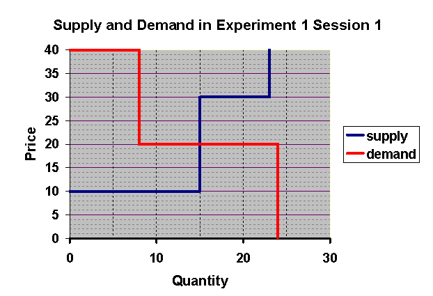
Figure 1.1 below shows the competitive supply and demand curve and the competitive equilibrium price and quantity in Session 1 with a class 47 students. As we see from the graph, the competitive equilibrium price is $20 and the competitive equilibrium quantity is 15 units sold.
Figure 1.1

Since individuals have very
limited knowledge of market conditions when they participate in the first
round, we would not expect all transactions to take place
at or close to the competitive equilibrium price. Nevertheless, the
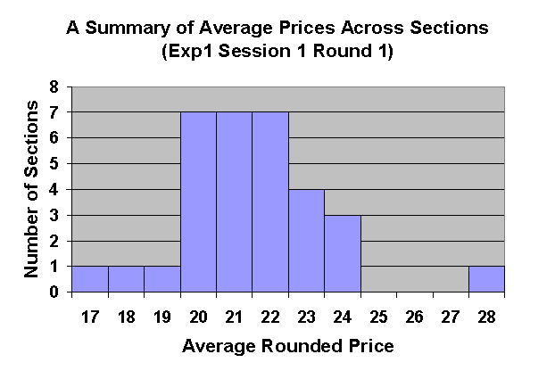
data shows that in the first round of Session 1, the average price
observed in most classrooms is strikingly close to the competitive
equilibrium price. This can be seen in Figure 1.2, which records
the distribution of mean prices across the 32 classrooms for which we have
data.
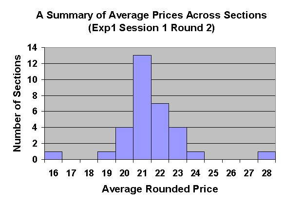
In the second round,
as traders learned more about the prices at which others bought and sold,
the mean prices in classrooms tended to cluster closer to the competitive
equilibrium price of $20, with mean prices remaining slightly higher than
the competitive price. This is shown in Figure 1.3
Figure 1.3
We have also recorded and
plotted the distribution of all recorded transactions in all sections.
In Figure 1.4, the purple line shows the distribution of transaction prices
in Round 1 and the yellow line shows the distribution in Round 2.
Notice that in round 1, there are large numbers of transactions at the
"focal" prices $15, $25, $30, and $35. In Round 2, the number of
transactions at these prices dimishes, while there is an increase in
the number of transactions that take place at prices close to the competitive
equilibrium price of $20.
Figure 1.4
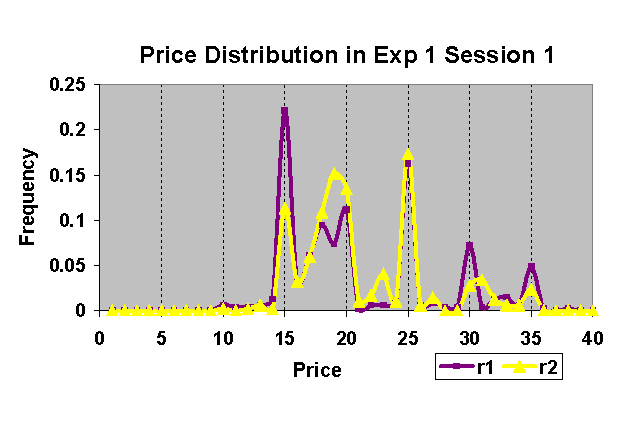
Figure 1.5
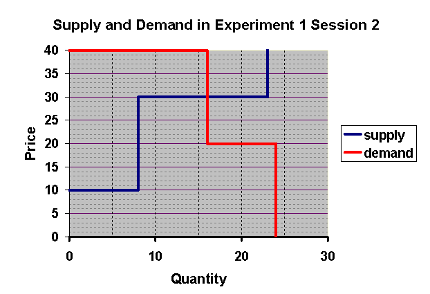
Figure 1.6
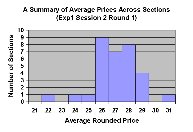
Figure 1.7
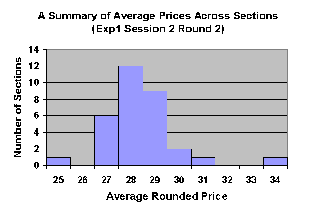
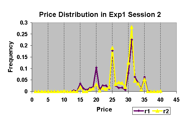
Figure 1.8 shows the distributions
of prices in individual transactions for each of the two rounds of Session
2. Notice that in Round 1 there are a significant number of transactions
at $20, which was the equilbrium price in Session 1 and that in Session
2, the number of such transactions decreases sharply, while
there is a corresponding increase in the number of transactions taking
place at prices close to $30, which is the Session 2 competitive equilibrium
price.
Figure 1.8
An alternative theory of
the events in these experiments is the following profit-splitting
hypothesis. Suppliers and demanders are paired at random.
In any pair for which the demander's buyer value exceeds the seller cost
of the seller, the demander and supplier will agree to a price halfway
between the demander's buyer value and the seller's seller cost.
If the demander's buyer value is less than the seller's seller cost, so
that no mutually profitable deal can be struck, then the buyer and the
seller will not transact and will search for another partner with whom
they can make a profitable trade.
In Session 1 of this
experiment, approximately 1/3 of the demanders have buyer values of $40
and 2/3 have buyer values of $20. Approximately 2/3 of the suppliers
have seller costs of $10 and 1/3 have seller costs of $30. If encounters
are random, then on average, 2/9 of the encounters will be between
demander with buyer value $40 and a supplier with seller cost
$10. According to the price-splitting hypothesis, they would
trade at a price of $25. About 1/9 of the random encounters
would be between a demander with buyer value $40 and a supplier with seller
cost $30. They would trade at a price of $35. About 4/9
the encounters would be between a demander with buyer value $20 and a
supplier with seller cost $10. They would trade at a price of $15.
Finally, about 2/9 of the encounters would be between a a demander with
buyer value of $20 and a supplier with seller cost $30.
These latter individuals would not trade. We see that in this market,
the only individuals who do not make a trade with the first person they
meet are demanders with $20 buyer values and suppliers with $30 seller
costs. Since everyone can make only one trade and since all of the low
cost sellers and high value demanders transact with the first person they
meet, those who fail to make a trade in their first encounter
will never find any mutually profitable trading opportunities.
Thus the profit-splitting hypothesis predicts that 7/9 of the traders will make trades. Prices paid will vary, depending on the buyer values and costs of the supplier and demander who happen to be matched. Under this hypothesis, approximately 28% (2/7) of all trades will take place at a price of $25, 14% (1/7) will take place at a price of $35, and 4/7 (56%) will take place at a price of $15.
In contrast, the competitive hypothesis predicts that about 2/3 of all traders will make trades and that all trades would occur at $20.
We see from Figure 1.4 that there is some support for the profit-splitting hypothesis, especially in the first round of trading. The graph of transactions in Round 1 has peaks at $35, $25, and $15. Moreover, as predicted by the profit-splitting theory, the most frequent price is $15. But there is also some support for competitive behavior. Contrary to the predictions of profit-splitting, about 30% of the transactions in Round 1 occur at prices in the range $18-20. In Round 2, the competitive hypothesis appears to gain at the expense of the profit-splitting hypothesis. In Round 2, the number of transactions at the extreme prices $35 and $15 decreases sharply, while the percentage of transactions occuring at prices within $2 of the competitive price increases from 30% to more than 40%.
We see from Table 1.8 that the profit-splitting hypothesis does not perform very well in explaining the results of either round of trading. Transactions at prices of $15 and of $35 are much less common than the profit-splitting hypothesis would predict.
In Round 1, about 35% and
in Round 2 about 50% of the transactions were at prices within $2 of the
competitive equilibrium price of $30. It is interesting to notice
that in Round 1, about 15% of the transactions took place at prices that
were approximately $20, the equilibrium price for Session 1 transactions.
Since prices in Round 2 of session 1 were typically clustered around $20,
this price appears to have been focal for many traders in the first round
of Session 2. In Round 2, market pressures seem to have erased
most of this effect. The proportion of transactions at
prices close to $20 fell to less than 5%.
In a unique competitive equilibrium, every transaction is profitable for at least one of the two traders and neither makes a loss. Competitive equilibrium is not the only outcome with this property. For example, assignment generated by random matching with profit splitting also has this property. As we demonstrated previously, random matching with profit splitting results in the expected number of transactions being about 7/9 of the number of traders, while competitie equilibrium results in a number of trades equal to just 2/3 of the number of traders.
Consider now an outcome in matchmaker arranges matchings so as to maximize the total number of supplier-demander pairs in which the demander's buyer value exceeds the seller's seller cost and requires these pairs to trade at some price profitable to both. For the distributions of buyer values and seller costs in this experiment, it is always possible to do this in such a way that every person in the market makes a trade at a profit.
Thus we have two examples of outcomes in which everyone makes a profit and the number of trades exceeds the number of trades in competitive equilibrium. These examples illustrate the following general theorem.
Theorem If there is a unique competitive equilibrium quantity, then if the number of trades is smaller than the competitive equilibrium quantity, there must remain at least one demander-supplier pair who have not traded, but could make a mutually profitable trade.
Proof: In a competitive equilibrium, every demander has a buyer value at least as high as the competitive equilbrium price and every seller has a seller cost no higher than the competitive equilibrium price. It follows that the buyer value of every demander who trades in competitive equilibrium is at least as high as the seller cost of every supplier who trades. Indeed if the competitive equilibrium quantity is unique, it must be that the buyer value of every demander who trades is higher than the seller cost of every supplier who trades.
Consider an allocation with
fewer trades than the number of trades in competitive equilibrium.
It must be that in this allocation, at least one of the suppliers who sells
in competitive equilibrium does not trade and at least one of the demanders
who buys in competitive equilibrium does not trade. From the result
of the previous paragraph, we see that the buyer value of this demander
is higher than the seller cost of at least one supplier who does not trade
in equilibrium. These two individuals could make a mutually profitable
trade.
QED
From this theorem, we see
that if traders understand their buyer values and seller costs and sufficiently
aggressive to find mutually profitable trade possibilities so long as such
exist, then the number of trades will be at least as large as the competitive
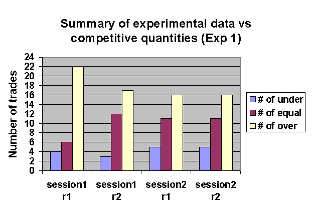
equilibrium quantity. We see from Figure 1.9 that there were
a few classes in which the number of trades fell short of the competitive
equilibrium quantity. In these classes it must be that at the end
of trading there remained at least one demander and at least one supplier
who did not trade but could make a mutually profitable trade with
each other. On the other hand, as our examples illustrate, it is
possible that trading leads to outcomes in which everyone who trades makes
a profit and where the number of trades exceeds the competitive equilibrium
number.
Experiment 2 (shifting supply) is an experiment in which a fixed quantity is produced at zero marginal cost, but the quantity shifts from one session to the next.
Experiment
3 (sales tax) is run first with no sales tax, then with a sales tax
collected from sellers and finally with a sales tax collected from buyers.